반응형
PatchmatchNet: Learned Multi-View Patchmatch Stereo
Introduction
- Multiview stereo 방법론 중 Patchmatch를 더 빠른 속도로 수행하기 위한 방법이다.
- occlusion, illumination changes, untextured areas, non-Lambertian surfaces등에 의해 난이도가 높은 문제이다.
- 현재의 방법들은 대체로 3D cost volume을 만들고, 이를 3D convolution으로 해결하려고 한다.
- 기존 방법 : R-MVSNet [43] decouples the memory requirements from the depth range and sequentially processes the cost volume at the cost of an additional runtime penalty. [7, 17, 41] include cascade 3D cost volumes to predict high-resolution depth map from coarse to fine with high efficiency in time and memory.
- 기존의 연산 속도 및 memory 문제를 deformable convolution을 활용한 cascade Patchmatch로 해결하고자 한다.
- Patchmatch idea into an end-to-end trainable deep learning based MVS framework. Going one step further, we embed the model into a coarse-to-fine framework to speed up computation.
- We augment the traditional propagation and cost evaluation steps of Patchmatch with learnable, adaptive modules that improve accuracy and base both steps on deep features.
- We estimate visibility information during cost aggregation for the source views.
- Moreover, we propose a robust training strategy to introduce randomness into training for improved robustness in visibility estimation and generalization.
Methods
- learning-based Patchmatch에서 coarse-to-fine framework를 활용하는 방식
- Multi-scale Feature Extraction
- FPN을 거쳐서 coarse to fine Patchmatch가 되도록한다

- Learning-based Patchmatch
- 과정은 다음과 같다.
- Initialization: generate random hypotheses.
- Propagation: propagate hypotheses to neighbors.
- Evaluation: compute the matching costs for all the hypotheses and choose best solutions
- Initialization 이후에는 Propagation -> Evaluation -> Propagation을 수렴할 때까지 수행한다.
- Propagation은 deep learning feature를 통해서 어떤 픽셀을 sample할 지 결정
- Evaluation은 visibility information을 예측하고, aggregate할 sample을 pixel neighbor에서 고른다.
- Unlike [3, 16, 38], we refrain from parameterizing the perpixel hypothesis as a slanted plane, due to heavy memory penalties. Instead, we rely on our learned adaptive evaluation to organize the spatial pattern within the window over which matching costs are computed

- Initialization and Local Perturbation
- 처음에는 random하게 depth를 selection한다.
- 한 픽셀마다 inverse depth range로 Df개 만큼의 interval로 depth를 고른다. 이를 통해 전체 depth range을 고르게 추정한다.
- local perturbation : k개의 stage에서 픽셀별로 Nk개의 hypothesis를 설정한다. 설정한 hypothesis range는 점차 줄여가는 식으로 refine한다.
- Hypothesis의 center는 previous iteration의 coarse feature를 upsample해서 결정한다.
- This delivers a more diverse set of hypotheses than just using propagation. Sampling around the previous estimation can refine the result locally and correct wrong estimates.
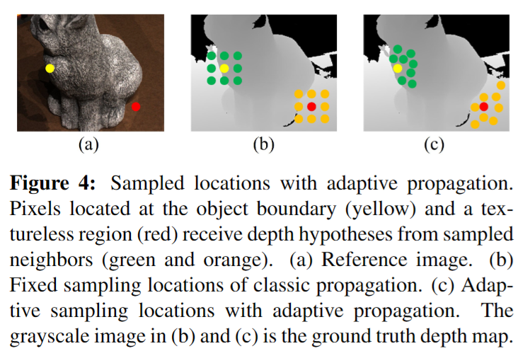
- Adaptive Propagation
- 같은 surface에 있으면 depth correlation이 강할 것이다. 이것을 활용하여 adaptive하게 propagation을 하려고한다.
- 이게 faster divergence의 핵심이다.
- Deformable convolution network를 사용해서 offset을 학습하고 bilinear interpolation으로 depth를 예측한다.

- Adaptive Evaluation
- differentiable warping, matching cost computation, adaptive spatial cost aggregation, depth regression으로 구성
- differentiable warping
- intrinsic/extrinsic matrix을 통해 corresponding pixel 계산
- warped source feature maps of view i and the j-th set of (per pixel different) depth hypotheses, Fi(pi,j ), via differentiable bilinear interpolation

- matching cost computation
- 여러 source의 information을 하나의 pixel로 합하는 것. 여기서는 visibility information을 활용
- the per group costs are projected into a single number, per reference pixel and hypothesis, by a small network.
- group similiarity는 다음과 같이 계산된다. F0는 reference, Fi는 source feature

- pixel-wise view weights wi는 pixel p의 image Ii에서 visibility information를 표현하는데 쓰인다. network를 하나 두고, Si를 input으로 들여 Pi를 per pixel, per hypothesis로 출력하여 아래와 같이 계산한다.

- final per group similarities는 다음과 같이 계산한다.

- 이후 1x1x1 convolution을 활용해서 single cost를 만든다.

- adaptive spatial cost aggregation
- 서로 다른 surface간의 aggregation 방지 목적
- 각 window의 pixel에 대해서 pixel offset을 학습한다.
- aggregated pixel cost는 다음과 같이 계산

- wk and dk weight the cost C based on feature and depth similarity
- 서로 다른 surface간의 aggregation 방지 목적
- depth regression
- C에서 softmax를 취해서 P를 얻고, 다음 식으로 Depth를 추정한다.

- C에서 softmax를 취해서 P를 얻고, 다음 식으로 Depth를 추정한다.

- Depth Map Refinement
- Patchmatch를 finest feature에서는 하지 않고 이전 coarse feature를 upsample하기만 한다.
- input depth map을 0~1 사이에만 두고 refine이후 다시 원래 scale로 되돌린다.
- FD, FI를 받아서 refine할 Depth residual을 계산한다.
- Loss Function
- L1 loss를 각 stage k에 대해서 수행한다. 이는 모든 depth estimation과 ground truth를 동원해서 계산한다.

- L1 loss를 각 stage k에 대해서 수행한다. 이는 모든 depth estimation과 ground truth를 동원해서 계산한다.
Experiments
- robust training strategy : 각 reference view마 4~10 개의 best view를 선정해서 학습. 이를 통해 generalization과 robustness 갖춰진다고 주장한다.
- Figure 6를 보면 thin한 물체에서 성능이 더 좋은데 그 이유를 adaptive propagation에 의한 것이라 주장

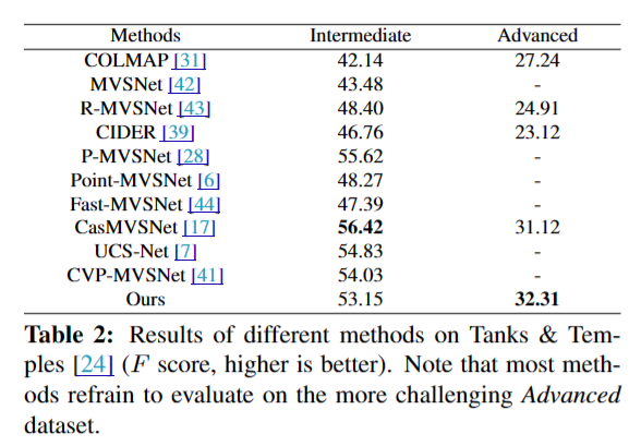
- 정량적 성능도 다른 method에 비해 크게 낮아지지 않았다는 것을 확인 가능하다.


- Figure 7 : 제안된 방법은 resolution이 커져도 다른 것들보다 더 빠르다. 메모리도 적게 먹는다. 물론 learning based 한정이다.
- Figure 8 : view weight를 통해서 covisible area를 잘 잡고 있다는 것을 알 수 있다.


- Abalation을 보면 위 메서드를 모두 사용했을 때 대부분의 dataset에서 좋은 성능을 보인다는 것을 알 수 있다.
- 또한, pixel-wise view weight & the robust training strategy 없이는 성능 낮아진다는 것을 확인했다.
- 그래프를 통해 convergence가 빠르다는 것을 보인다. 저자가 주장한 learned adaptive propagation이 여기에 도움이 된다는 주장.
- 또한 view 개수가 5개가 가장 좋다고 보였다.


반응형